CAPEX vs OPEX Diagnosis with Work Sampling
Use activity findings to assess investment and operating alternatives without promising automatic financial returns.
Updated:
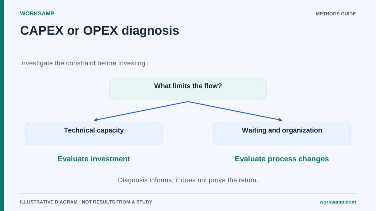
Introduction: The Plant Investment Dilemma
Every year, operations directors and plant engineers face a critical financial crossroads: allocate the budget to CAPEX (new machines, automation, expansions) or to OPEX (process optimization, maintenance, training). This decision, often based on intuition or the pressure to modernize, can lead to million-dollar investments that fail to address the root cause.
The most common scenario is a production line that falls short of its targets. The immediate perception is: "We need a faster machine." However, what the data might reveal is that machine sits idle 40% of the time waiting for material, or that operators spend more time looking for tools than producing. Without objective evidence, a new asset is purchased (CAPEX) to solve a problem that is, in fact, an organizational one (OPEX).
This is where Work Sampling becomes a fundamental diagnostic tool. It delivers an objective, statistically robust, and non-invasive X-ray of the plant, enabling investment decisions grounded in evidence rather than assumptions.
What is Work Sampling and why is it key for your plant?
Work Sampling is a technique for analyzing time distribution based on a simple yet powerful principle: statistical inference. Instead of timing activities continuously (which can be costly and alter behavior), a large number of instantaneous observations (known as Snap Readings) are taken at random moments across days or shifts.
The scientific foundation: From the binomial to the Gaussian curve
Each observation records which activity category an operator or piece of equipment falls into at a given instant. Are they producing, adjusting, waiting, or in maintenance? As hundreds of these "photographs" accumulate, the proportion of observations in each category approaches the true proportion of time dedicated to that activity.
This process rests on the binomial distribution (success/failure for each category) and, thanks to the Central Limit Theorem, its results can be expressed with the precision of the Gaussian curve. This allows us to calculate not only a percentage but also a confidence interval (e.g., "Productive time is 35% ± 3% with 95% confidence"), bringing scientific rigor to the conclusions.
Main advantage and bias control
Structured observations reduce reliance on recall but do not remove subjectivity, misclassification, incomplete coverage or reactivity. Random times support the selection design; they do not guarantee unpredictability or provide a measured Hawthorne correction.
WorkSamp is aimed at planning and recording random observations; Cronometras is aimed at direct time studies. Product functions are not transferred by ecosystem membership.
WorkSamp Methodology: Step-by-step for a reliable diagnosis
Carrying out a Work Sampling study with rigor follows a structured process across three key phases.
Phase 1: Study design with statistical rigor
Before stepping onto the shop floor, defining the analytical framework is essential.
- MECE Taxonomy (Mutually Exclusive, Collectively Exhaustive): A closed list of activity categories is created that covers 100% of what can be observed and where each one is unique. A typical example might be:
- Active Production (direct added value)
- Adjustment / Setup
- Corrective / Preventive Maintenance
- Internal Logistics (fetching materials, moving parts)
- Waiting (for instructions, upstream breakdowns)
- Break / Personal
- Sample Size Calculation (N): The number of observations required for the results to be significant is determined. The statistical formula is:
N = (Z² * p * (1-p)) / e²
Where Z corresponds to the confidence level (1.96 for 95%), p is the estimated proportion of the most critical activity, and e is the acceptable margin of error (e.g., ±5%). There is no universal standard count: p=0.5, z=1.96 and e=0.05 give 385 independent visits after rounding up; e=0.03 gives 1,068. Correlated rounds and stratum-specific estimates require design review.
Phase 2: Execution of the random observations
With the design ready, the analyst performs visits following the random sequence generated (Tippett). On each visit, within a matter of seconds, they classify what they observe according to the MECE taxonomy. The key lies in randomness and the immediacy of the Snap Reading. And to complement the analysis with staff working hours, platforms such as Induly, specialized in working-time monitoring, provide the timekeeping records the user can export and cross-reference with the observation data.
Phase 3: interpret a proportion without turning it into a cause
Define direct work and its denominator. A low share may reflect logistics, safety requirements, task mix, reserve capacity or conditions outside the observed person’s control. No verified 35–40% threshold here diagnoses an OPEX problem.
OEE requires matching data: A=run time/planned production time; P=(ideal cycle time×total count)/run time; Q=good count/total count. State observations provide context but do not by themselves measure cycles or product quality. See the OEE calculation.
From data to decision: CAPEX or OPEX
The true value of the study emerges when the results are interpreted in the context of investment.
Teaching scenario 1: investigate organization
Assume 28% direct work, 30% logistics and 15% waiting, with no attribution to a real customer. The remaining 27% needs classification before interpreting the whole. The figures prompt questions about supply, sequence and support; they do not prove that another machine is unnecessary.
Compare tool organization, scheduling, training and layout alternatives. Improvements may be capital or operating expenditure depending on their accounting nature; CAPEX/OPEX is not simply equipment versus organization.
Teaching scenario 2: investigate equipment constraints
A 75% direct-work share and failures concentrated on an asset can justify investigating repair, replacement or extra capacity. They do not select CAPEX on their own. Assess demand, bottlenecks, safety, quality, life-cycle cost, maintenance and sensitivity scenarios.
A hypothetical 30% result with a ±2.5-percentage-point 95% margin would require approximately 1,291 independent observations when planning with p=0.30. Without n and design, that interval cannot be attached to a plant. Narrow intervals do not establish causality or financial return.
Conclusion: Modern productivity is built on data, not assumptions
Sampling provides descriptive evidence for comparing hypotheses and alternatives. It does not establish automatic production-system integration or guarantee a return. The financial decision needs demand, cost and risk analysis as well as time allocation.
Before approving the next CAPEX budget, put your operation through a Work Sampling diagnosis. The answer may surprise you and redirect your resources to where they will actually generate returns: the intelligent optimization of what you already have.
Resources and Tools
To dive deeper into these methodologies and find specialized solutions, the ASETEMYT directory is an essential starting point:
- Explore time-and-motion analysis solutions in the ASETEMYT Directory.
- To add your tool or service to the directory, visit Add to ASETEMYT.
- Discover more articles on industrial productivity in the ASETEMYT Blog.
- Check out specific tools such as Cronometras for time studies or Induly for real-time working-time monitoring.