Work Sampling and Continuous Improvement with PDCA

Introduction

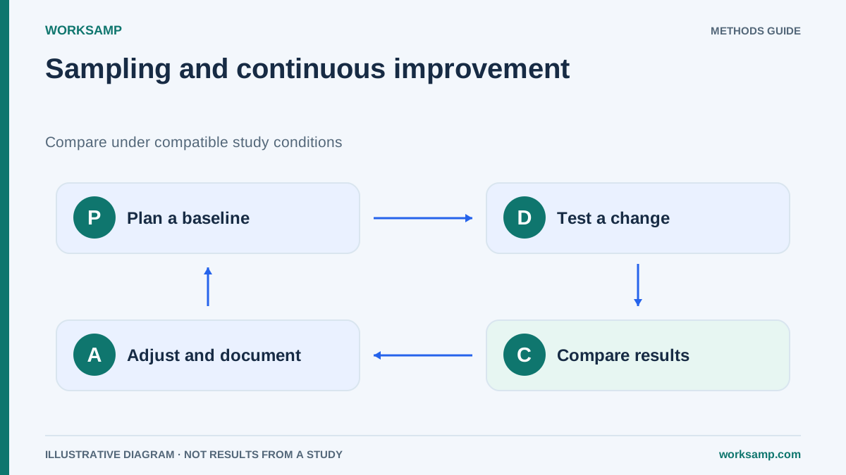
PDCA organises improvement into plan, do, check and act. Sampling can estimate activity shares for comparisons across periods. It does not by itself attribute observed changes to an intervention.

This guide combines design, fieldwork and comparison using two simulated examples. Statistical uncertainty, comparability and practical relevance are assessed separately.

In this guide we will explore how to integrate work sampling studies into each of the four phases of the Deming cycle in a practical way, with an illustrative application case, formulas, common mistakes, and implementation recommendations.

What is Work Sampling and why does it fit with PDCA?

Work Sampling is an instantaneous and random observation technique that allows determining the proportion of time that operators, machines, or processes dedicate to different activities (productive, unproductive, delays, etc.) without the need to time every second. Its validity rests on three pillars:

Planning must cover the target population and period, minimise classification bias and consider dependence and weighting. Randomisation does not guarantee independence. The simple formulas below assume independent Bernoulli observations and an adequate normal approximation.

Mathematically, the required sample size is calculated with the formula:

N = (Z² · p · q) / S²

Where:

Z = value of the normal distribution associated with the confidence level (1.96 for 95%, 2.58 for 99%).
p = estimated proportion of the activity of interest (for example, productive time).
q = 1 − p.
S = acceptable absolute error (precision).

Sampling produces a structural datum: the statistical photograph of how time is distributed in a process. That photograph is precisely the input PDCA needs so that each iteration is an informed decision and not a leap in the dark.

The PDCA cycle: why does it fail without data?

The PDCA cycle, popularized by W. Edwards Deming based on Walter Shewhart's work, is an iterative method with four phases:

Plan: diagnose the problem and design the improvement.
Do: implement the improvement on a small scale.
Check: measure the effect of the improvement.
Act: standardize if the improvement worked, or adjust and return to Plan.

The classic failure in industry occurs when the Check phase is replaced by perceptions or biased data:

"The operator goes faster now" → subjective perception.
"The supervisor says the line performs better" → confirmation bias.
"It looks better in the video" → sample of a single instant.

An interval expresses uncertainty under the design assumptions; it does not eliminate bias or confounding.

An estimate and interval describe sampling uncertainty; they do not turn before/after observation into causal certainty.

1. Plan: the baseline with sampling

Before proposing any improvement, you have to know where you stand. A work sampling study executed at the beginning of the PDCA project provides the baseline with which results will be compared.

Recommended procedure:

Define the target population (line, cell, team, section).
Estimate a pilot proportion p₀ (for example, p₀ = 0.55 if you believe 55% of time is productive). If you have no idea, you can use p₀ = 0.5 (most conservative case, which maximizes p·q).
Calculate N with the formula already indicated, setting a confidence level (95% or 99%) and an acceptable absolute error (for example, ±3 or ±5 percentage points).
Distribute the N observations over the days of the study, respecting randomness (random routes and schedules).
Record each observation in a MECE category (Mutually Exclusive, Collectively Exhaustive): Productive, Unproductive, Delay, Setup, etc.

At the end, you obtain a percentage per category with its standard error σₚ = √(p·q/N) and a confidence interval that describes the uncertainty of the measurement.

Numerical example:

If after 800 observations 480 productive ones have been recorded, then:

p̂ = 480 / 800 = 0.60 (60% productive)
σₚ = √(0.60 · 0.40 / 800) = √(0.0003) = 0.0173 (1.73%)
95% Interval: 0.60 ± 1.96 · 0.0173 = [0.566; 0.634] → [56.6% ; 63.4%]

Compare periods by estimating their difference and its uncertainty. Requiring the new proportion to fall outside the first period's individual interval is not a general hypothesis-test rule.

2. Do: implement the improvement at a controlled scale

Observation during implementation is also possible if learning or incidents are part of the objective. If a run-in is excluded, justify and document its duration before seeing results and state the time scope of the conclusion.

Document the exact date and time of the start of the intervention.
Define the "run-in" period (typically 1–2 weeks) to avoid measuring learning effects.
Isolate other variables that may confound the result (lot change, new staff, etc.).

Controlling variables and documenting the intervention improves interpretation but does not guarantee causality. Consider demand, mix and comparison groups, and disclose design limitations.

3. Check: validate the improvement with new sampling

This is where work sampling is deployed again, this time post-intervention. The goal is to compare the new proportion with the baseline in a statistically valid way.

Procedure:

Compare samples with compatible populations, categories and conditions. For two large independent samples, estimate Δ = p̂₁ − p̂₀ and its unpooled standard error:

SE(Δ) = √[p̂₀(1−p̂₀)/n₀ + p̂₁(1−p̂₁)/n₁]

An approximate normal 95% interval is Δ ± 1.96 SE(Δ). Excluding zero provides evidence of a difference under the assumptions. An equality test may use the pooled proportion under the null. Clusters, paired data or autocorrelation require a different analysis.

Continuation example:

After the intervention, in a new study of 800 observations, 552 productive ones are recorded:

p₁ = 552 / 800 = 0.69 (69%)
95% Interval: [0.658; 0.722] → [65.8% ; 72.2%]

In this simulated example, Δ = 0.69 − 0.60 = 0.09. The approximate difference interval is 4.3 to 13.7 percentage points. It supports a period difference under the model; it does not prove that the intervention caused it.

4. Act: standardize or iterate

Decide whether to extend, modify or stop the change using effect size, uncertainty, quality, safety, cost and feasibility. Non-significance does not establish no effect; precision may be insufficient.

Sampling informs the decision but does not make it automatically or replace process knowledge.

Simulated practical case: reducing dead time in an assembly line

Context. A household appliance plant executes a PDCA cycle on a manual assembly line of 8 operators, with an 8-hour shift. (An example built for didactic purposes; it does not correspond to a real WorkSamp deployment or to any specific client.) Management suspects that delays due to material search (tools, parts, documentation) are inflating unproductive time.

Plan Phase – Baseline. A sampling study is designed:

Confidence level: 95% → Z = 1.96.
Pilot estimate: p₀ = 0.50 (conservative case, no prior data).
Acceptable error: S = ±4% → S² = 0.0016.

N = 0.9604 / 0.0016 = 600.25; rounding up gives 601 planned observations. Suppose 600 valid records are eventually obtained. The model’s approximate worst-case margin becomes 4.001 percentage points rather than exactly 4; the following example uses that achieved sample.

After 600 random observations over 5 days (120 per day, with randomized routes and schedules), the following results are obtained:

Category	Observations	Proportion
Productive	306	51.0%
Unproductive	78	13.0%
Delays (material search)	144	24.0%
Delays (others)	54	9.0%
Setup	18	3.0%

The 95% confidence interval for Material Search Delays is:

p = 0.24, q = 0.76, N = 600.
σₚ = √(0.24 · 0.76 / 600) = √(0.000304) = 0.0174.
CI 95%: 0.24 ± 1.96 · 0.0174 = [0.206; 0.274] → [20.6% ; 27.4%].

On a compatible eight-hour base, the interval corresponds to approximately 1 h 39 min–2 h 12 min per person-shift as an aggregate average. It does not describe every individual or establish realizable savings.

Do Phase. A bounded improvement is implemented:

Workstation reorganization with tools and parts in shadow boards.
Start-of-shift checklist procedure.
Labeling and fixed location of consumables.

Run-in period: 2 weeks (not measured).

Check Phase – Post-intervention. Sampling is repeated under the same conditions: N = 600, identical taxonomy, 5 days.

Category	Observations	Proportion
Productive	366	61.0%
Unproductive	72	12.0%
Delays (material search)	90	15.0%
Delays (others)	54	9.0%
Setup	18	3.0%

Comparison of Material Search Delays:

p₀ = 0.24 → CI [20.6%; 27.4%].
p₁ = 0.15 → σₚ = √(0.15·0.85/600) = 0.0146 → CI [12.1%; 17.9%].

Material-search waiting changes from 24% to 15%: −9 points, with an approximate change interval of −13.5 to −4.5 points under independent sampling. Work classified as productive rises from 51% to 61%: ten points correspond to 48 minutes on an eight-hour base, not proven extra output or margin. Demand and other changes may explain some of the difference.

Act. The scenario proposes a further pilot before expansion to four other lines. Check comparability and risks, and choose follow-up according to the decision and precision needed; 60 days is a scenario option, not a rule.

Common mistakes when integrating sampling and PDCA

Define the required effect and precision before collection.
Record missing data and dependence without inflating effective size.
Keep categories comparable or document a validated mapping.
Investigate demand, mix and staffing changes.
Separate significance, causality and economic relevance.
Monitor quality and safety rather than optimising a single proportion.

Frequency and design of follow-up samplings

Follow-up should be designed for the change that matters. A monthly sample of 200 may help but cannot establish absence of regression and has lower precision than 600 comparable records.

P-charts require comparable subgroup definitions and an adequate binomial model. Weight the centre line by records and vary limits when n changes; signals prompt investigation rather than identify the cause automatically.

Follow-up can trigger a new improvement hypothesis when a signal warrants investigation.

Conclusions and recommendations

Work Sampling does not compete with PDCA: it underpins it. While the Deming cycle provides the iterative framework for improvement, sampling provides the statistical evidence that each phase needs to be more than a good intention.

The keys to a successful integration are:

Plan confidence, precision and coverage together.
Estimate differences using a design-appropriate method.
Do not use overlap of individual intervals as a universal criterion.
Check causes and financial effects with additional data.
Adapt monitoring and charts to actual size and dependence.

PDCA and sampling can improve decision traceability when assumptions and limitations are communicated. A statistical difference is one part of evaluation, not a guarantee of success.

Resources and Tools

WorkSamp: Work Sampling studies with random observation and sample-size calculation.
Cronometras: Time analysis of the tasks to be standardised.
Induly: Industrial time and attendance tracking to contextualise working days and shifts.
ASETEMYT Directory: Professionals and companies in methods and time engineering.
ProdCont: Industrial productivity consulting; comprehensive operational audits (not just work sampling) for plants with several open fronts.

Sources

NIST: confidence intervals for proportions. NIST: p-charts.